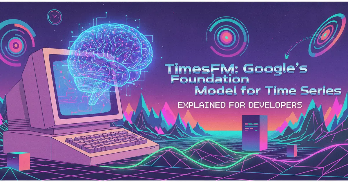
TimesFM proposes a different deal: skip the training step entirely.
It is a pretrained model from Google Research that forecasts time series it has never seen before. Same idea as an LLM, except instead of predicting the next word, it predicts the next value. You hand it a NumPy array of history, tell it how far ahead to look, and get a forecast back. No training loop, no hyperparameter search.
This post covers what it actually does, how the API feels, and what landed in the brand-new 3.0 release.
The mental model: patches are tokens
An LLM chops text into tokens and learns to predict the next one. TimesFM chops a time series into patches (contiguous windows of 32 time steps) and learns to predict the next patch.
That is basically the whole idea. A decoder-only transformer, the same family as GPT, pointed at numbers instead of text.
Patching matters for two practical reasons. Attention cost grows with sequence length, so grouping 32 points into one token keeps long histories affordable. And a patch captures a local shape (a weekly cycle, a spike, a slow drift) as a single unit, which is closer to how time series actually behave than treating each individual point as a token.
The training data is the other half of the story. TimesFM was pretrained on a corpus of over a trillion time points spanning retail, finance, web traffic, energy, and synthetic data. It has seen enough patterns of “sales-shaped thing” and “traffic-shaped thing” that when you hand it yours, it recognizes the family. That is what makes zero-shot forecasting work.
You also get uncertainty for free. The model outputs 9 quantiles (10th through 90th percentile) at every step, not just a single line. If you have ever had to bolt confidence intervals onto a forecast after the fact, this is a real convenience.
Getting started
Installation is a one-liner:
pip install timesfm[torch]Or from source with uv:
git clone https://github.com/google-research/timesfm.git
cd timesfm
uv venv && source .venv/bin/activate
uv pip install -e .[torch]
The 2.5 API
This is the API most tutorials and existing code use. You load a checkpoint, compile it once with a config, then call forecast():
import torch
import numpy as np
import timesfm

torch.set_float32_matmul_precision("high")

model = timesfm.TimesFM_2p5_200M_torch.from_pretrained(
    "google/timesfm-2.5-200m-pytorch"
)

model.compile(
    timesfm.ForecastConfig(
        max_context=1024,
        max_horizon=256,
        normalize_inputs=True,
        use_continuous_quantile_head=True,
        force_flip_invariance=True,
        infer_is_positive=True,
        fix_quantile_crossing=True,
    )
)

point_forecast, quantile_forecast = model.forecast(
    horizon=12,
    inputs=[
        np.linspace(0, 1, 100),
        np.sin(np.linspace(0, 20, 67)),
    ],
)

point_forecast.shape     # (2, 12)
quantile_forecast.shape  # (2, 12, 10)
Two things worth noticing. The inputs are plain 1D arrays and they do not have to be the same length, which is genuinely nice when you are forecasting a batch of products with different histories. And a few config flags do real work: infer_is_positive stops the model predicting negative sales, fix_quantile_crossing prevents the 60th percentile landing below the 40th.
Swapping in your own data is the boring part, which is the point:
import pandas as pd

df = pd.read_csv("weekly_demand.csv", parse_dates=["week"])
values = df["demand"].values.astype(np.float32)

point, quantiles = model.forecast(horizon=52, inputs=[values])
That is a 52-week forecast with prediction intervals, from a CSV, with no training.
What changed in 3.0
TimesFM 3.0 landed in late August 2026, and it is a bigger jump than the version number suggests.
Every checkpoint through 2.5 was strictly univariate. One series, its own history, nothing else. That is a real limitation, because most forecasting problems in the wild are not like that. If you are forecasting ice cream sales, past sales alone miss the picture: related product sales matter, foot traffic matters, and crucially, the promotion you already scheduled for next Tuesday matters.
3.0 is natively multivariate. It brings three things that were previously awkward or impossible:
- Multiple targets. Forecast several related series jointly and let the model use the correlations between them.
- Past covariates. Features you only know historically, like last month’s foot traffic.
- Past-future covariates. Features you know in advance, like scheduled promotions, holidays, or a weather forecast.
That last one is the interesting capability. The model learns the promotion-to-sales relationship from your historical context, then applies it to future days where you have a promotion planned. A univariate model just projects the weekly pattern forward and misses the bump entirely.
Architecturally, 3.0 does this with alternating attention. Tokens attend horizontally across time (strictly causal, so no leakage from the future), then vertically across series at each time step, so the model can learn how a spike in one series relates to another. Those two layers alternate through the stack.
It also stopped decoding autoregressively. Earlier versions generated one patch at a time, which meant latency and compounding errors over long horizons. 3.0 appends masked placeholder tokens for the whole future window and fills them all in a single forward pass.
The 3.0 API is different from 2.5, so this is not a drop-in upgrade:
import numpy as np
from timesfm3 import TimesFM3Evaluator, ModelConfig

config = ModelConfig(
    checkpoint_path="google/timesfm-3.0-pytorch",
    per_core_batch_size=16,
    device="cuda",
)
forecaster = TimesFM3Evaluator(config)

context_len, horizon = 128, 24

target = np.random.randn(3, context_len).astype(np.float32)
past_only_cov = np.random.randn(3, context_len).astype(np.float32)
The multivariate architecture and single-pass decoding make 3.0 substantially more capable for real-world forecasting tasks, at the cost of a migration from the 2.5 API. For new projects, 3.0 is the version to start with.